Lab 12: Path Planning and Execution

Waypoint Path and Overall Strategy

The predefined waypoints were used directly as the high-level path for this lab. The robot started from (-4, -3) and followed the waypoint sequence until it reached the final target near (0, 0). The green line in Figure 1 shows the planned route, while the white lines show the walls and obstacles in the mapped environment.

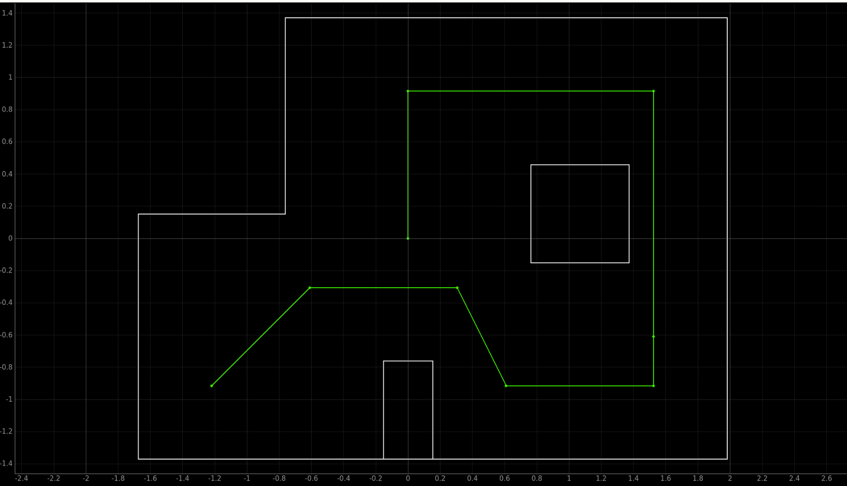
I implemented an offboard waypoint-following strategy. The Python notebook stored the waypoint list, computed the required heading and distance for each segment, and sent the corresponding BLE commands to the robot. The Artemis board then executed the low-level motion onboard, including IMU-based turning and forward movement. This structure allowed the high-level planning logic to remain easy to debug in Python while keeping the time-sensitive motor control on the robot.

WAYPOINTS = [
    (-4, -3),
    (-2, -1),
    (1, -1),
    (2, -3),
    (5, -3),
    (5, -2),
    (5, 3),
    (0, 3),
    (0, 0),
]

For each pair of consecutive waypoints, the robot used a turn-and-move primitive. First, the notebook computed the desired heading from the current waypoint to the next waypoint. Then it sent a turn command to the robot. After the robot completed the turn, it moved forward toward the next waypoint and stopped before starting the next segment. Selected Bayes localization was also included at key waypoints to reduce accumulated pose error.

Robot Implementation and Tuning Process

Arduino code modification

The Arduino program served as the onboard low-level motion controller. It received BLE commands from the Python notebook and executed the corresponding motor actions on the robot. The main commands used in this lab were ORIEN_PID_CONTROL for turning, FORWARD for forward motion, and STOP for stopping the robot. This design allowed the Python notebook to handle high-level waypoint planning, while the Artemis board handled time-sensitive motor execution.

enum CommandTypes {
  GET_TOF_IMU,
  PID_POSITION_CONTROL,
  ORIEN_PID_CONTROL,
  FORWARD,
  STOP,
  REQUEST_DATA,
  MOVE_TOF_DELTA,
};

For orientation control, the robot used IMU/DMP-based yaw feedback. The laptop sent a relative target angle, and the Artemis board ran an onboard PID loop to rotate the robot in place. At the beginning of each turn, the current yaw was saved as the zero reference. The robot then continuously compared the current yaw with the target yaw and adjusted the motor output until the yaw error became small enough.

case ORIEN_PID_CONTROL:
{
    float Kp, Ki, Kd, target_delta_yaw;
    bool success = true;

    success &= robot_cmd.get_next_value(Kp);
    success &= robot_cmd.get_next_value(Ki);
    success &= robot_cmd.get_next_value(Kd);
    success &= robot_cmd.get_next_value(target_delta_yaw);

    if (!success) {
        return;
    }

    stop();
    delay(200);

    float yaw_zero = 0.0f;
    read_dmp_yaw_latest(yaw_zero);

    float target_yaw = wrap_angle_deg(target_delta_yaw);
    unsigned long start_time = millis();

    while (millis() - start_time < 5000) {
        float yaw_abs_now;
        if (!read_dmp_yaw_latest(yaw_abs_now)) {
            continue;
        }

        float current_yaw = wrap_angle_deg(yaw_abs_now - yaw_zero);
        float yaw_rate = get_gyro_z_dps();

        int u = pid_orientation_control(
            Kp, Ki, Kd,
            current_yaw,
            target_yaw,
            yaw_rate
        );

        spin_in_place(u);

        float err = wrap_angle_deg(target_yaw - current_yaw);

        if (fabs(err) <= 5.0f && fabs(yaw_rate) < 20.0f) {
            break;
        }
    }

    stop();
    break;
}

This turning method was more reliable than open-loop timed turning because the robot used yaw feedback to close the loop. I also included a time cutoff in the turning loop. This prevented the robot from being stuck in the PID loop if the desired angle could not be reached exactly due to wheel slip or sensor noise.

I also modified the FORWARD command so that it could accept both a motor speed and a duration. This change was necessary for the pulsed forward strategy used later in the Python notebook. Instead of sending one long forward command, the notebook could send multiple short forward pulses, each with a limited duration.

case FORWARD:
{
    int speed;
    int duration_ms = 300;

    bool success = true;
    success &= robot_cmd.get_next_value(speed);

    if (!success) {
        return;
    }

    bool got_duration = robot_cmd.get_next_value(duration_ms);
    if (!got_duration) {
        duration_ms = 300;
    }

    if (duration_ms < 0) {
        duration_ms = 0;
    }

    if (duration_ms > 500) {
        duration_ms = 500;
    }

    forward(speed);
    delay(duration_ms);
    stop();

    tx_estring_value.clear();
    tx_estring_value.append("FORWARD_DONE|");
    tx_estring_value.append(speed);
    tx_estring_value.append("|");
    tx_estring_value.append(duration_ms);
    tx_characteristic_string.writeValue(tx_estring_value.c_str());

    break;
}

The command format became speed|duration_ms. The duration was capped at 500 ms as a safety mechanism. This was important during debugging because it prevented the robot from continuing to drive forward for too long if a command was not tuned correctly. This modification made the forward movement safer and easier to adjust experimentally.

The original ToF-based distance controller was kept as an optional local movement primitive. It computes a target ToF value by subtracting the desired forward displacement from the initial ToF reading. However, during waypoint navigation, ToF readings did not always correspond to the actual displacement along the planned path.

int initial_tof = read_tof_mm();
int target_tof = initial_tof - distance_mm;

if (target_tof < 60) {
    target_tof = 60;
}

This ToF-based method worked only when the robot had a stable wall reference in front of it. If the robot faced open space, a corner, or an angled surface, the ToF value could change unpredictably. Therefore, the final path execution relied mainly on waypoint-based pulsed forward commands and selected Bayes correction.

Python code modification and tuning process

The Python notebook implemented the high-level waypoint planner. It stored the waypoint list, computed the desired heading and distance for each segment, and sent BLE commands to the robot. In my coordinate convention, 0° points along the positive y direction, and 90° points along the positive x direction. Therefore, I used atan2(dx, dy) to compute the desired heading.

def wrap_to_180(angle_deg):
    while angle_deg > 180:
        angle_deg -= 360
    while angle_deg < -180:
        angle_deg += 360
    return angle_deg


def execute_segment(p0, p1, previous_heading=0.0, segment_id=None):
    x0, y0 = p0
    x1, y1 = p1

    dx = x1 - x0
    dy = y1 - y0

    # Heading convention:
    # 0 deg = +y direction, 90 deg = +x direction
    desired_heading = math.degrees(math.atan2(dx, dy))
    turn_angle = wrap_to_180(desired_heading - previous_heading)

    distance_cells = math.sqrt(dx * dx + dy * dy)
    distance_mm = distance_cells * CELL_SIZE_MM

    send_turn(turn_angle)
    time.sleep(0.4)
    send_stop()
    time.sleep(0.3)

    send_move_pulsed(distance_mm)

    send_stop()
    time.sleep(0.2)

    return desired_heading

This function was the basic motion primitive for one waypoint segment. The notebook first computed the desired heading and relative turn angle, then sent the turning command to the robot. After the turn finished, the robot moved forward using the pulsed forward motion function. The returned heading was used as the previous heading for the next segment.

During early testing, I found that one long continuous forward command could easily cause overshoot or collision. This was especially true when the battery voltage changed or when the robot entered the longer segments in the second half of the path. To make the motion more controllable, I replaced long forward commands with short forward pulses.

FORWARD_PWM_SAFE = 55
ROBOT_SPEED_MM_S_SAFE = 250.0
MAX_PULSE_MS = 500
PULSE_GAP_S = 0.05
DISTANCE_SCALE = 0.55


def send_forward_pulse(speed=FORWARD_PWM_SAFE, duration_ms=300):
    duration_ms = int(min(duration_ms, MAX_PULSE_MS))
    duration_ms = max(0, duration_ms)

    payload = f"{int(speed)}|{duration_ms}"
    ble.send_command(CMD.FORWARD, payload)

    time.sleep(duration_ms / 1000.0 + 0.15)

    send_stop()
    time.sleep(PULSE_GAP_S)


def send_move_pulsed(distance_mm):
    commanded_distance = max(0.0, distance_mm * DISTANCE_SCALE)
    remaining = commanded_distance

    while remaining > 0:
        max_pulse_distance = ROBOT_SPEED_MM_S_SAFE * MAX_PULSE_MS / 1000.0
        pulse_distance = min(remaining, max_pulse_distance)
        pulse_ms = int(1000.0 * pulse_distance / ROBOT_SPEED_MM_S_SAFE)

        send_forward_pulse(FORWARD_PWM_SAFE, pulse_ms)

        remaining -= pulse_distance

    send_stop()

The parameter DISTANCE_SCALE was tuned experimentally. Since the robot does not have wheel encoders, the same PWM and pulse duration do not always produce the same physical displacement. The actual travel distance depends on battery voltage, wheel slip, floor friction, and motor response. The pulsed strategy made the robot safer during testing, while DISTANCE_SCALE allowed me to correct the average distance error.

After the basic pulsed motion worked, I tuned the path segment by segment. The first half of the route became very accurate with the global parameters above. However, the segment from (2, -3) to (5, -3) consistently moved slightly too far. Instead of changing the global distance scale, I applied a local correction only to this problematic segment.

# Segment 4: (2,-3) -> (5,-3)
# This segment tended to overshoot, so I used a smaller local scale.

old_scale_seg4 = DISTANCE_SCALE

DISTANCE_SCALE = old_scale_seg4 * 0.85

prev_heading = execute_segment(
    (2, -3),
    (5, -3),
    previous_heading=prev_heading,
    segment_id=4
)

DISTANCE_SCALE = old_scale_seg4

This local tuning step was important because the earlier segments were already accurate. Reducing the global distance scale would have made those segments too short. Applying the correction only to Segment 4 improved the final path without affecting the successful parts.

The later part of the route was more challenging because it contained long straight segments. In particular, (5, -2) -> (5, 3) and (5, 3) -> (0, 3) amplified small heading errors. I first tried one-cell subsegments, which were accurate but too slow. The final version used approximately two-cell subsegments, together with a mildly conservative distance scale and shorter pulse gaps.

old_distance_scale = DISTANCE_SCALE
old_max_pulse_ms = MAX_PULSE_MS
old_pulse_gap_s = PULSE_GAP_S

# Mild conservative mode for later long segments
DISTANCE_SCALE = old_distance_scale * 0.90
MAX_PULSE_MS = min(old_max_pulse_ms, 600)
PULSE_GAP_S = 0.03

long_segment_6_points = [
    (5, -2),
    (5, 0),
    (5, 2),
    (5, 3),
]

for k in range(len(long_segment_6_points) - 1):
    prev_heading = execute_segment(
        long_segment_6_points[k],
        long_segment_6_points[k + 1],
        previous_heading=prev_heading,
        segment_id=f"6.{k+1}"
    )

    send_stop()
    time.sleep(0.35)

# Restore original parameters
DISTANCE_SCALE = old_distance_scale
MAX_PULSE_MS = old_max_pulse_ms
PULSE_GAP_S = old_pulse_gap_s

This tuning process balanced speed and accuracy. One-cell stepping made the robot very accurate but too slow, while commanding the full long segment at once caused large overshoot. The two-cell subsegment strategy was a practical compromise for the final video run.

Selected Bayes localization

To reduce accumulated pose error, I also integrated selected Bayes localization into the path execution framework. Instead of localizing after every waypoint, I used localization flags to decide when the robot should stop and update its pose estimate. This followed the idea that localization is most useful after segments where dead-reckoning error is likely to accumulate.

LOCALIZE_FLAGS = [
    False,  # waypoint 0: (-4,-3), start
    True,   # waypoint 1: (-2,-1)
    False,  # waypoint 2: (1,-1)
    False,  # waypoint 3: (2,-3)
    False,  # waypoint 4: (5,-3)
    True,   # waypoint 5: (5,-2)
    True,   # waypoint 6: (5,3)
    True,   # waypoint 7: (0,3)
    True,   # waypoint 8: (0,0)
]


if LOCALIZE_FLAGS[i + 1]:
    localized_pose = run_bayes_localization(current_pose_hint=current_pose)

    current_pose = (
        target_xy[0],
        target_xy[1],
        localized_pose[2]
    )

In the final implementation, Bayes localization was used conservatively. The heading estimate from the Bayes result was used to correct the robot's orientation estimate, while the x-y position was snapped to the target waypoint. This avoided an issue observed during testing: if the noisy Bayes x-y estimate was used directly, the computed distance for the next segment could become too large and cause the robot to move too far.

def execute_segment_from_pose(current_pose, target_xy, segment_id=None):
    x0, y0, previous_heading = current_pose
    x1, y1 = target_xy

    dx = x1 - x0
    dy = y1 - y0

    desired_heading = math.degrees(math.atan2(dx, dy))
    turn_angle = wrap_to_180(desired_heading - previous_heading)

    distance_cells_raw = math.sqrt(dx * dx + dy * dy)
    distance_mm_raw = distance_cells_raw * CELL_SIZE_MM

    if segment_id is not None and 1 <= segment_id < len(WAYPOINTS):
        nominal_p0 = WAYPOINTS[segment_id - 1]
        nominal_p1 = WAYPOINTS[segment_id]

        ndx = nominal_p1[0] - nominal_p0[0]
        ndy = nominal_p1[1] - nominal_p0[1]

        nominal_distance_mm = math.sqrt(ndx * ndx + ndy * ndy) * CELL_SIZE_MM

        DISTANCE_CAP_RATIO = 1.15
        max_allowed_distance_mm = DISTANCE_CAP_RATIO * nominal_distance_mm

        distance_mm = min(distance_mm_raw, max_allowed_distance_mm)
    else:
        distance_mm = distance_mm_raw

    send_turn(turn_angle)
    time.sleep(0.4)
    send_stop()
    time.sleep(0.3)

    send_move_pulsed(distance_mm)

    send_stop()
    time.sleep(0.3)

    estimated_pose = (x1, y1, desired_heading)

    return estimated_pose

The distance cap made the Bayes correction more stable on the physical robot. It allowed the current pose and heading to be corrected, but prevented a noisy localization estimate from causing an unexpectedly long motion command. Overall, the final implementation was the result of repeated testing: pulsed forward motion improved safety, segment-specific scale correction improved local accuracy, two-cell subsegments improved the later long portions of the path, and selected Bayes localization helped reduce accumulated orientation error.

Results

Early failed trial

Before the final successful run, I tested several earlier versions of the path execution strategy. Video 1 shows one representative failed trial. In this attempt, the robot reached the area near (5, 3), but its stopping position was too far forward. As a result, when it tried to execute the next segment from (5, 3) to (0, 3), the robot did not have enough clearance for the left turn and collided with the wall.

This failure was useful because it revealed that the main problem was not the waypoint sequence itself, but the accumulated execution error in the later part of the route. The front half of the path was already fairly accurate, but long straight movements in the second half caused small distance and heading errors to accumulate. Once the robot stopped too far forward near (5, 3), the next turn became unsafe.

To address this issue, I modified the later part of the route. First, I avoided commanding the full long segments as one motion. Instead, I split the long movements into shorter subsegments. Second, I used a mildly conservative distance scale for the later segments so that the robot would not overshoot as much. Third, I locally reduced the distance scale for segments that repeatedly moved too far. These changes made the later turns safer and improved the repeatability of the full path.

Final successful run

Video 2 shows the final successful run. In this version, the robot completed the full waypoint route without manual assistance, without wall collision, and stopped near the final target (0, 0). The stopping accuracy was better in the first half of the route, where the waypoint distances were shorter and the accumulated error was smaller. In the second half, the robot still had small deviations from the ideal waypoint locations, but the adjusted segment-specific parameters and shorter subsegments prevented the robot from colliding with the walls.

Although the robot did not stop exactly at every ideal waypoint, the final run satisfied the main objective of the lab. The robot followed the planned waypoint sequence, completed the full path, avoided collisions, and finished close to the final target. Therefore, I considered this run a successful path planning and execution demonstration.

Discussion

The early failed trial showed that the main challenge was accumulated execution error in the later part of the route. The robot stopped too far forward near (5, 3), so the following left turn toward (0, 3) did not have enough clearance and resulted in a wall collision. This happened because the later straight segments were longer, and small heading or distance errors were amplified over several grid cells. Since the robot did not have wheel encoders, forward displacement depended on PWM, command duration, battery voltage, wheel slip, and floor friction.

To solve this problem, I kept the original tuned parameters for the accurate front half of the route, applied a local distance-scale reduction to segments that tended to overshoot, and split the longer later segments into shorter subsegments with a mildly conservative setting. Selected Bayes localization was also used conservatively: the heading estimate was used for orientation correction, while the x-y position was snapped to the current target waypoint to keep the next commanded distance stable. With these changes, the final run completed the full route without manual assistance or collision and stopped near (0, 0), although small deviations from the ideal waypoint locations remained in the later part of the path.